5. Improving the Setup¶

The first months of my time spent on the Nikhef/KVI Proton Radiography project overlapped with the previous student working on it, Tsopelas (2011). The first test run with protons was in November 2011 at the AGOR cyclotron at KVI. The results from this test run are the basis of my work on the project. Any problems or issues were the things I would work on and improve in my time at Nikhef, which will be discussed in this chapter.

5.1. Results from November and Overview¶

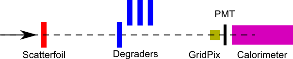
Figure 1: A schematic of the proton detector setup as installed at AGOR. From left to right: the beam enters the experimentation room at 150MeV. A lead scatterfoil of 1.44mm thickness broadens the beam and reduces the energy to 145.5MeV. In total the beam passes through about 3m air, reducing the energy down to 143MeV. The aluminium degraders can be remotely moved into or out of the beam. On the right hand side the GridPix tracker, the trigger scintillator (PMT) and the $BaF_2$ calorimeter are represented.

Apart from establishing the efficacy of the setup in the situation of a proton accelerator, the performance of the GridPix was profiled and the calorimeter calibrated as well as profiled. The main objective of the endeavor is to image objects. To test this, we collected data in the following configurations:

Changing the full beam energy with aluminium absorbers in order to provide an energy calibration for the calorimeter. The experimentation room provided remotely movable aluminium plates, which we varied between between 20, 40, 57 and 61mm, corresponding to an energy (at the detector) of 118, 88.3, 54.8 and 44.4MeV.
The aim of the setup is to reconstruct objects in the beam, so a very simple object was placed in the beam: up to four copper plates covering half of the detector. The four plates were each 2.7875mm thick.
Two copper wedge shapes with different angles provided a more complex test of our ability to reconstruct objects. The dimensions were 30x30x12mm and 30x30x24mm.

A thorough analysis of the GridPix, and a preliminary analysis of the calorimeter during these runs may be found in Tsopelas (2011). We attained an event acquisition rate of about 2Hz, due to a frequent loss of synchronicity between the tracker and calorimeter acquisition systems.

The calorimeter performance in particular presented us with some challenges, as we found discrepancies between the runs. Using the aluminium absorbers we intended to calibrate the energy response of the calorimeter. Also, the full beam should be calibrated precisely, because the energy deposited in the object is calculated by subtracting the calorimeter energy from the full beam. Throughout the day the full beam (143.6MeV) was measured with the calorimeter, but unfortunately the measurements did not always correspond with each other. Tsopelas mentioned that a possible cause could be temperature, but after further study it was found that the full beam calorimeter response variation correlates well with changes in proton rate. The AGOR proton beam operates at a fixed 55MHz frequency, but allows tuning the number of protons per bunch. Because initially synchronicity was lost after only a few events, the effective proton rate was lowered to about 0.5 - 1 kHz, meaning that most bunches would be empty, and the nonempty bunches would be filled according to some Poisson distribution. After discussion with dr. Tjeerd Ketel, a Nikhef calorimeter expert, the rate sensitivity of the calorimeter was deemed the most probable cause of the shifts in the calorimeter response. The shifts were found to be the same for peak position and peak integral. To reconstruct the wedges, the data taken from the copper plate runs were therefore used to calibrate the calorimeter response, as these runs were performed at a similar proton rate. The calibration curve is seen in figure 3.

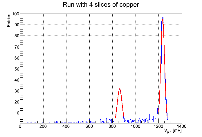
Figure 2: The calorimeter response for the 4 copper slice run. Two peaks are visible, the left corresponding to the protons that went through the copper and the right corresponding to the full beam. Both peaks are fitted with a gaussian, and correspond to points in figure 3.

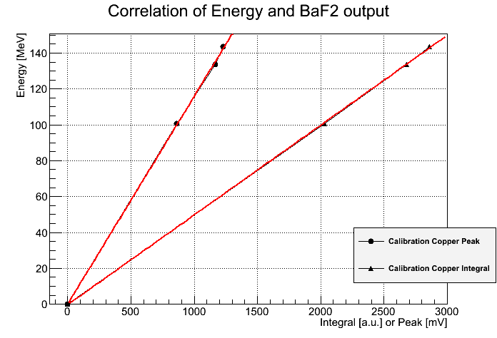
Figure 3: By fitting a gaussian over a histogram of all data points with 1 plate of copper, 4 plates of copper, and full beam, the calorimeter response for that particular energy was obtained (see figure 2). The fits were tested for stability by altering the range to which the gaussian would fit. This fit is only accurate for a capture rate of ~1kHz. The fit is linear, as expected.

About 30 tracks for each wedge each were selected by hand, because an algorithm for automated event selection was not available at the time. Event selection is required, because we have seen problematic events such as double tracks, $\delta$ -electrons in the drift volume, and curved tracks. For a proper analysis, these need to be filtered, and either fitted differently or be discarded. For now, some events were selected where the projection of the track in the plane transverse to the beam was a clean and compact blob: straight single proton tracks without complications. Using the NIST tables (National Institute of Standards and Technology, 2011) for protons in copper, the wedges were reconstructed. Fitting the data was done using both peak position and peak integral, and both with a free first order polynomial and one with a fixed slope, based upon the known dimensions of the wedges. The peak position fitted data agrees best with the known slope.

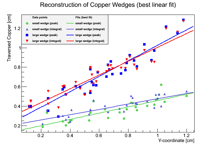
Figure 4: The analysis of the reconstruction of the wedges. The plotted points are traversed copper paths as function of transverse coordinate. These are reconstructions using either the integral of a calorimeter response curve of simply its peak height. Also plotted are the best linear fits. It appears the integral derived wedge reconstruction has a less steep slope than the peak derived wedge reconstruction. The slopes are for the large wedge 0.79 (peak) and 0.71 (integral), and for the small wedge 0.32 (peak) and 0.27 (integral).

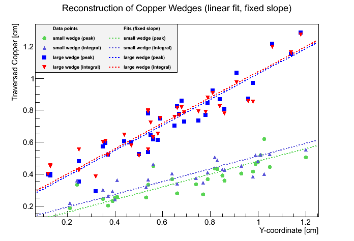
Figure 5: The analysis of the reconstruction of the wedges. The plotted points are traversed copper paths as function of transverse coordinate. These are reconstructions using either the integral of a calorimeter response curve of simply its peak height. Here fits with a fixed slope are plotted, taken from the actual slope of the wedges. Now the integral derived reconstruction results in slightly thicker wedges. The actual slopes are 0.40 and 0.80 for the small and large wedges respectively.

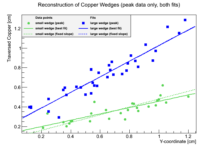
Figure 6: The analysis of the reconstruction of the wedges. Only the peak reconstructed points are shown. Straight lines are best linear fits, dotted lines are fits with the slope set to the known value. The slope of the free fit corresponds best with the known slope for the peak derived points. Only for the thin wedge are the slopes different between the two fits. The large wedge fitted slope (0.79) agrees very well with the real slope (0.80), while the small wedge fitted slope (0.32) diverges a bit from the actual value (0.40).

These results (figures 4, 5, 6), together with the analyses of the GridPix and calorimeter, prove the concept works. The limited event set, due to the lack of event selection, precludes us from doing a meaningful statistical analysis, so error bars are omitted for now. The main issues discovered are loss of synchronicity, low event acquisition rate, a small loss of hits up to 1mm above the grid, supposedly due to trigger delays (figure 5.7 in (Tsopelas, 2011)), and an unknown sensitivity to rate of the calorimeter. Most of my time was spent in solving these problems and it was decided to focus on four points:

An improved calorimeter, with more stability. A small literature study is performed to establish whether or not such a calorimeter exists and is available for purchase.
A new trigger design that can keep synchronicity better and perhaps solve the missing hits 1mm above the grid. The GridPix readout system, RelaxD, with the associated software, RelaxDAQ, has a readout limit of 120Hz. A trigger system that can keep up with such a rate is therefore investigated. Usage of the RelaxD busy signal is planned so that dead time during readout is minimized further.
Timestamps on both the tracking data and calorimeter data would help, because in case one system missed a trigger and the other not, the timestamps could be used to filter the incomplete events and still allow the remaining events to be used. Although not a must-have, it would make the data acquisition more fault tolerant. Also, new software for the RelaxDAQ readout already provides nanosecond timestamping.
An improved data acquisition system for the calorimeter. We had been using a digital oscilloscope, which due to limited buffers could only store a small number of events, resulting in very short data taking runs. Nanosecond precision timestamping would provide an independent method of ensuring synchronization.
An increased number of GridPix chips, so as to increase the drift volume and thereby the tracking volume. In addition, to improve the fitting accuracy and therefore object reconstruction performance, it would be advantageous to have separate trackers before and after the object.
Event selection, so that the analysis and statistics can be improved. Problematic tracks should be filtered and handled separately.

5.2. Towards pCT¶

Our 1.5cm cubed tracker does not live up to the demands of medical professionals quite yet. As mentioned in chapter 3, recreating the typical 30cm squared projection would require us to scan over that area in some fashion, or keep the tracker aligned with the beam. Because this is time consuming or not very practical, a larger tracker is the desired alternative. Another improvement is to add a second tracking plane. As seen in chapter 4, most setups feature multiple tracking planes. Since the GridPix tracks in 3D, there is no reason to have multiple planes close to each other. Far apart is however again advantageous, in particular before and after the patient or object, to correct for scattering inside the imaging volume. For our setup this means that we want to put a number of GridPixes alongside each other inside the same gas volume, which then would not be cubical anymore but extended in the transverse dimension. This ‘slab’ should be repeated, once before and once after the patient. The increased tracking volume results in a larger detection area and thus a faster imaging process. Unfortunately, our GridPix broke down, so a new one had to be constructed. A new batch of TimePix chips that arrived at the Detector R&D group proved to be of lesser quality, and most had to be discarded, which meant that the multi-GridPix was not possible at this time. One single-chip GridPix replacement was created, with a gas volume with the same height as before but wider dimensions around the chip. In the sides of the GridPix casing metallic leads serve as field shapers. Close to the field shapers the field is not quite uniform, so putting the walls of the gas volume outwards improves the fields uniformity above the chip, but keeps the effective drift volume the same. The gas volume changed from about 1.5cm cubed to 3cm x 3cm x 1.5cm. The new TimePix chip has been confirmed to work, but because of the bad batch was assumed to be sensitive to strong HV fields. Previously a $CO_2-DME$ (50%-50%) mixture had been used, which is known to provide a reasonable middle ground between drift velocity and diffusion. It requires a comparatively high potential between anode and cathode to ionize however, so another gas mixture was selected that allows for lower potentials at the cost of more diffusion: Helium-Isobutane (80%-20%). The minimum track-generating drift potential was experimentally obtained by placing a beta emitter close to the GridPix and increasing the potential until tracks became visible. Using Magboltz, a CERN software package to simulate the transport of electrons in gas mixtures, the drift velocity was obtained.

5.2.1. Fitting curves¶

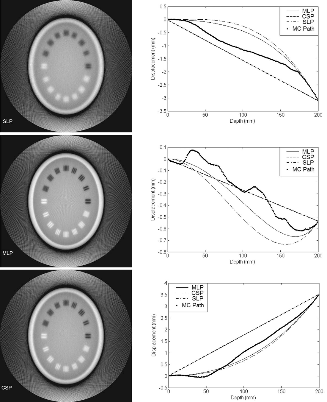
Figure 7: Left column: Fully reconstructed phantoms using three algorithms. In the center left MLP is used, and this algorithm is often seen as the most successful for academic purposes. Right column: Different fitting algorithms are compared to the simulated track of a proton (thick line). Algorithm abbreviations: SLP, MLP, and CSP. Images courtesy of Li et al. (2006).

Fitting curves to the recorded proton tracks is a part of the analysis not yet performed. The procedure can be broken up in two parts: fitting tracks within the GridPix drift volume and fitting through the imaged object.

Fitting GridPix.

In the November test run, the GridPix was aligned with the beam line, and any tracks that were not straight were discarded. This resulted in a spot on the projection on the transverse plane, which circumvented any fitting difficulties. A proper analysis, especially when scattered, non-aligned tracks are reconstructed, requires a robust fitting method. Within the Detector R&D group, the master thesis of De Nooij (2009) may serve as a starting point for an actual implementation of a reconstruction algorithm. Of particular interest will be the alignment between multiple GridPix planes, as that is proving rather complicated elsewhere in the R&D group.
Fitting objects.

Literature shows that most groups dealing with proton imaging use a Most Likely Path method (Hurley et al., 2012, Li et al., 2006, Penfold et al., 2009, Cirrone et al., 2007, Bashkirov et al., 2009, Cirrone et al., 2007, Depauw and Seco, 2011, Talamonti et al., 2010), which involves known entry and exit points, and knowledge of the interaction of the particle with tissue (figure 7). In X-ray CT reconstructions are often implemented using FBP or IR methods. FBP is based on Radon transformations, which is a method of deconvolving the projection that the calorimeter measures into an series of coefficients (integral), which correspond to the different tissues that the beam passed through. For these coefficients a model of the body or organ is used to provide an ansatz for the transformation, and so a possible solution is derived. In IR this process is repeated in order to decrease noise and increase medical information as much as possible. The trade off is between speed and precision. For pCT most groups speak of an ART, which is similar to IR approaches. This stage of data processing was never reached so no implementation has been built as of yet, but the references may be used to see where the competition is.

5.3. Calorimeter¶

In the November test run we had placed two objects in the setup, with the intention of attempting to reconstruct them from the data. These objects were two triangular wedges of different size. The way we planned to reconstruct the wedges was by correlating the pixel data perpendicular to the beam and the calorimeter output. In calibrating the calorimeter it became apparent that the output was sensitive to changes in beam rate. The beam rate had changed a few times, and after repeatedly trying to create a calibration curve that agrees with common knowledge on PMTs, it was clear that the datasets taken at different beam rates are not compatible: one cannot (easily) compare between the two. The known temperature dependence was considered (Schotanus and Eijk, 1985), but since the environmental temperature was monitored and found to be stable, it was rejected as a significant factor in performance.

Because of the above reasons, and because the calorimeter is an old device that was not used and maintained for over 10 years, the use of another calorimeter was considered. The point of the calorimeter is to measure the residual proton energy, and $BaF_2$ does not compare well to other crystals on its energy resolution. At Nikhef an F101 crystal was found available. This crystal was created for the HERMES experiment, for which Nikhef supplied the PMTs attached to these crystals. In order to see if the new crystal could be suited for our setup, a study was done on the penetration depth of protons using simulation software Geant4. Protons of 190MeV were found to reach a depth in F101 and $BaF_2$ to within a few percent of each other. The F101 crystal was large enough to capture such protons, but about its use in proton capture no information was found. At KVI a spare PMT was found, the XP2242B, and I looked into coupling it to a $LaBr_3$ crystal, as at KVI the combination had been used with satisfaction. Figure 8 shows the resulting light yield of such a combination. Connecting the PMT to the crystal turned out to be problematic, because it was hygrofobic. Moreover, again not much on proton capture performance was known, making it unclear whether this combination would be an improvement over the $BaF_2$ .

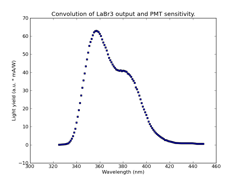
Figure 8: The convolution of the XP2242B PMT and $LaBr_3$ response. Sources: Photonis (None), Shah et al. (2004).

Since the sensitivity to particle rate is a main concern with the $BaF_2$ calorimeter, we decided that we needed to be sure about such details before any calorimeter purchase. For $LaBr_3$ we could not find such data, putting that crystal on the list of uncertain performers. We could find data on Helium capture performance with Cesium doped YAP/YAG. At this point, the decision was made to move the focus towards the calorimeter acquisition system, as that could be independently researched from the calorimeter. Also, the fast output of the $BaF_2$ crystals was a trait not found in any other crystal, and is advantageous because it reduces the number of required secondary scintillators in the beam for a coincidence trigger, reducing the problem of scattering. For the record, table 5.1 contains all data found on crystals in calorimetry.

For a future search, the following points must be taken into consideration:

Decay constant: how fast is the signal? For higher rates, the decay constant must be shorter. Also, a secondary fast peak like $BaF_2$ displays is very useful as input for a trigger system.
Energy resolution. The point of the calorimeter is energy measurement, so the error should be as small as possible. Ideally, the resolution is known for protons in the 50-200MeV range.
Performance dependence on factors such as rate, temperature, etc.
Emission wavelength is ideally in a range easily captured by PMTs.
Radiation hardness.

Comparison of materials for calorimetry.¶
Material	Density [g/cm3]	Emission maximum [nm]	Decay constant	Conversion efficiency	Energy resolution	Remarks
$NaI$ $(Tl)$	3.67	415	0.23 ms	100		Radiation sensitive, Hygroscopic
$CsI$ $(Tl)$	4.51	550	0.6/3.4 ms	45	0.6% @He 45MeV	Radiation sensitive, Hygroscopic
$CsI$ $(Na)$	4.51	420	0.63 ms	85		Hygroscopic
$CsI$	4.51	315	16 ns	4 - 6
$CaF_2$ $(Eu)$	3.18	435	0.84 ms	50
$^6LiI$ $(Eu)$	4.08	470	1.4 ms	35		Hygroscopic
$^6Li$ glass	2.6	390 - 430	60 ns	4 - 6
$CsF$	4.64	390	3 - 5 ns	5 - 7		Hygroscopic
$BaF_2$	4.88	315, 220	0.63 ms, 0.8 ns	16, 5	~9%
$YAP$ $(Ce)$	5.55	350	27 ns	35 - 40	2.7%
$GSO$ $(Ce)$	6.71	440	30 - 60 ns	20 - 25	2.3% @He 45MeV	Resolution for 1H similar
$BGO$	7.13	480	0.3 ms	15 - 20	2.9% @He 45MeV	Rad. Hard., Res. for 1H similar
$CdWO_4$	7.90	470 / 540	20 / 5 ms	25 - 30		Radiation hard
Plastics	1.03	375 - 600	1 - 3 ms	25 - 30
$F101$	3.86			see (Kolsteinb et al., 1996)	6.6% @1GeV	Radiation hard
$YAG$ $(Ce)$		50	70 ns		3.00% @He	Res. for 1H similar
$LaBr_3$ $(Ce)$	5.06	360 - 380	25 ns		2.7-3%	Temp. insensitive, Noisy, Hygroscopic

Sources: (Scionix, 2012, Kolsteinb et al., 1996, Cirrone et al., 2007, Shah et al., 2004, Schotanus and Eijk, 1985, Novotny, 1998, Novotny and Doring, 1996).

5.4. Calorimeter Data Acquisition¶

Using an oscilloscope for data acquisition, even an advanced one, turned out to be suboptimal. The main problem with our device was the limited internal buffer that required the operator to reset the measurement every half minute. A system able to continuously readout the calorimeter is desirable. The other requirements are that it be able to cope with acquisition rates of at least 100Hz, and that it has a history buffer allowing for look back at the moment of trigger. Of course the device has to support an external trigger. A feature that would be nice to have is a timestamp with better than microsecond precision.

The device suitable as CaloDAQ was found in the HiSparc project (HiSparc, 2012). HiSparc is a network of cosmic ray detectors in the Netherlands, placed at high schools throughout the country. The number of HiSPARC detection sites in the Netherlands is approximately 100, and they are used to reconstruct the particle showers caused by cosmic rays. The hardware is designed to be cheap and consists of a set of scintillators coupled to a computer. One single device digitizes the scintillator outputs, tests for a coincidence and sends the sampled signal to a computer, on which the results may be viewed and uploaded to a central server. The project is coordinated from the HiSparc group at Nikhef, and both hardware and software are developed at Nikhef. The device used to hook up the scintillators to the computer is called the HiSPARC-box, and this is the device we chose to use as well.

5.4.1. The HiSparc ADC¶

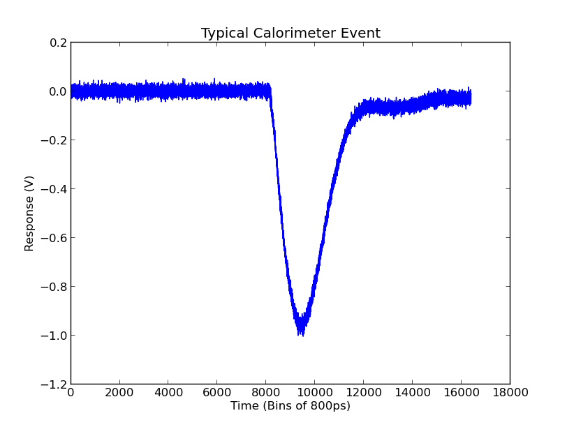
Figure 9: A typical curve recorded with the digital oscilloscope in the test run at KVI in November 2011. This oscilloscope samples at 1.25GHz, resulting in a time period per sample of 800ps. The event window is 13μs. This data was resampled to see the effect of lower sample rates on the error in peak height, see figure 10. The noise on the baseline before the peak is seen as the convolution of the ADC quantization error and the noise of the calorimeter itself. Assuming a gaussian distribution, this noise is calculated at $\sigma = 0.0135V$ .

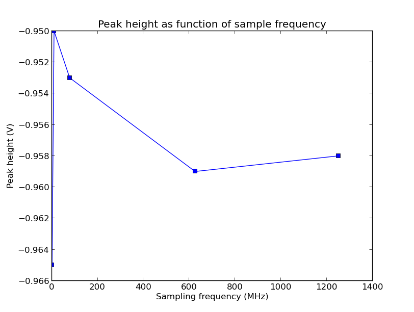
Figure 10: Here the peak height is plotted as a function of sampling frequency. The curve in figure 9 is resampled to obtain the various frequencies plotted here. The peak height is taken from a second degree polynomial fit around the top of the peak. It can be seen that the variation even at 1.2MHz is 0.7% of the peak height at the original 1.25GHz sampling rate, and less than the convolution of the ADC quantization error and the noise of the calorimeter itself, which is $\sigma = 0.0135V$ . For a sampling rate of 400MHz the difference is of the order of 0.1%.

The HiSPARC-box version 3 has the following characteristics:

Two ADCs continuously sampling at 200MHz are run in antiphase to give an effective sampling rate of 400MHz. Each sample corresponds to a time period of 2.5ns and is sampled at 12 bits. Given the 0-2.5V input range of the ADCs, this results in a precision of $1.25*10^{-12}$ V/bin, which falls well below the noise threshold observed in the data in figure 9: $\sigma = 0.0135V$ . To get an estimate on whether the sampling rate will suffice, the peak height is studied as function of the sample rate. Figure 10) shows that changing to a sampling rate of 400MHz would introduce an error smaller than the error due to other factors.
The two ADCs need to be aligned because uncalibrated they will have a different response due to being different chips.
A dynamic range of about 2.5V. Amplitudes from the $BaF_2$ calorimeter were between 0 and -1.5V, so this is a perfect fit.
The interface between the computer and the HiSparc-box is a USB2 connection and occurs via a custom message protocol. Software on the computer can send messages to the USB driver, which then transmits them to the HiSparc-box: a write action. Conversely, a read action can be performed by the computer that causes the USB driver to request the contents of the device buffer. The structure of the custom message protocol is defined in a manual.
A buffer sized at 40k samples, translating to 10µs of history. The length of an event can be set to anything that fits in this window. The device will store event data in the buffer, according to definable parameters such as trigger condition and the number of samples that constitutes an event. This event window is set in terms of a number of samples pre-trigger and post-trigger. Upon a request for the buffer contents, the contents is moved out of the buffer and into the computer. If no readout requests are made, the buffer will fill up and the device will halt storing events until memory is freed.
Although the device has two channels available for analog to digital conversion, only one is currently used. A future possibility is to use analog electronics to integrate the peak signal and use the second channel to capture this integrated signal. Potentially this could result in a higher acquisition rate, as presumably less samples are required to sample the integral compared to the full curve.
Because of the inclusion of the buffer, reads and writes may occur simultaneously. This means that a readout does not imply dead time. A read action remove that data from the buffer, freeing space for new acquisitions. If data is written (acquired) faster than it is read, the device will block new acquisitions until read actions free some memory, resulting is an effective dead time. Reasons for this to occur may be high trigger rates or a large event window.
In the HiSparc experiment the trigger is a coincidence between the two channels, but an external trigger is available. Theoretically the only limit to the trigger rate is the sampling frequency, so there is no reason to assume the desired 100-120Hz is a problem.
Because of the distributed nature of the HiSparc experiment and the need to couple shower data between stations, each HiSparc-box has a GPS unit which provides a calibration point every second to the internal HiSparc clock. An extra nanosecond clock inside the unit is reset every second when the GPS signal is received, resulting in the internal HiSparc clock to achieve nanosecond precision for the timestamps it attaches to every event message. This provides the extra check for synchronicity.

5.4.2. Development of custom software¶

We have seen that the hardware specifications of the HiSparc-box are equal or better than what we are looking for, but the software requires discussion as well. In the HiSparc project the box is accompanied by an extensive software package. A lot of analysis is performed on site, at each station, by this software. This allows for both a local view for high school students and saves bandwidth when uploading the data to the central server. While this software is comprehensive, it is fairly slow and relies on commercial software for which the Detector R&D group has no license. The event rate of a typical HiSparc station is 1-4Hz, and the software can keep up with an acquisition rate of approximately 10Hz. This is mostly due to the single-threaded nature of the software and the amount of computation required for analysis. Also, the software is designed with an always online internet connection in mind, to upload the data. Only some statistics are saved locally. These were reasons enough to not use this software, but to write a custom program.

A major part in the development of our own custom software was the driver: in the standard HiSparc program it had been implemented inside the runtime of the commercial LabView package, which connected directly to the USB device. I started the software task with an investigation into rewriting this driver without using the commercial runtime. Being coded in C using LabView libraries, initially such a port was deemed feasible. Because it was designed to work on the Windows operating system, the first attempt was to get the code to compile within Microsoft Visual Studio. After some attempts this was abandoned in favor of a Python binding for the official manufacturers driver for the chip inside the HiSparc-box. Although the message protocol would have to be reimplemented, this option was deemed more suitable to exploratory programming and less complicated to achieve. A HiSparc derived device called Muonlab, built for muon detection by high school students, already had a software implementation built with the Python binding. Apart from the (undocumented) requirement to load the firmware first, the HiSparc-box could be interfaced with the computer in a similar fashion. Because the manufacturer provides drivers for both Windows and Linux, this provided the option to use either. The rule of thumb is that RelaxDAQ attains higher rates under Linux due to a more suitable scheduler, making the potential move to Linux advantageous.

Encouraged by this success, the HiSparc group at Nikhef revived their own old plan to have a Python-environment for testing. They proceeded to write their own implementation of the HiSparc communication protocol, but now based on a combination of libusb (authors, 2012) and PyFTDI (authors, 2012), a driver for the chip written in Python itself, interfacing directly with the USB device via libusb. This approach, titled PySparc (Fokkema and Laat, 2012), turned out to be equally successful, and a comparative study on the performance of both implementations yielded similar acquisition rates at similar event window settings (10μs versus 13μs), indicating that the hardware was the limiting factor and not the Python-environment, known for ease of use but not numerical performance.

So, two basic implementations were produced, comparable in performance in first instance. In addition, the HiSparc group wrote a comprehensive message parser, a ADC calibration routine and a firmware-loader. These last two have Windows-only equivalent tools, built by the HiSparc hardware group.

5.4.3. Online message parsing and speedup¶

The point of the new CaloDAQ is synchronized acquisitions at a high rate, so both implementations were tested in order to determine the best option. Time was spent on the separation of readout and data-processing into separate threads or processes. Transferring data out of the HiSparc-box buffer into the computer is a matter of calling a read-function as often as possible; a classic example of a pull architecture. Its result is a stream of bytes which need to be decoded into messages according to a message protocol. Using the HiSparc message parser to process the acquisition data in the same thread as receiving the acquisition data consistently led to slowdowns: the HiSparc-box buffer was filling up faster than the software could read, causing the HiSparc-box to start missing events. The continuous readout loop should therefore be as light as possible and do not much more than transfer the data to computer memory where another process or thread can take as long as it needs to decompose the bits into meaningful data. Since Python does not support true multithreading (spreading threads over multiple CPU-cores) but only emulates it, a multiprocessing variant was investigated for both implementations. Multiprocessing in Python works by simply starting multiple Python interpreter processes tasked with whatever function is delegated to each process. The API is fortunately very similar between threading and multiprocessing. It was quickly unconvered that my own implementation could not make use of multiprocessing due to the Python binding using Ctypes to interface with the manufacturers driver. This driver is simply a compiled library (.dll or .so), which can’t be shared by the multiple processes created by Python. Python however seems to enforce access to all resources for all processes, even if they don’t use them, but it can’t fork the single USB resource. The PySparc implementation also lost control over the readout process with multiprocessing. Within the HiSparc group a suitable explanation could not be found, but it was firmly established that it didn’t work.

A secondary benefit of multiple threads or processes is the ability to spin out the readout loop from the main program, allowing it to accept user interrupts upon which the readout could be stopped. This is why the (emulated) multithreading API was used in the final implementation. The other major design decision was to simply write all data directly and continuously to disk, allowing for offline processing by the PySparc message parser. A few extended data taking runs with both implementations showed that the implementation with the manufacturers driver resulted in extraneous bits and missed hits (compared to a separate counter). A modified PySparc implementation was therefore chosen as our default. Three side-effects are that PySparc includes a routine to align the ADCs and one to upload the firmware, voiding the use of two Windows-only utilities. The third side-effect is that the HiSparc group experienced problems running the code on Windows, although the creator of the Python bindings reports that there should be no objections. It successfully runs on MacOSX and Linux, which is good enough, considering the better supposed performance of RelaxDAQ in Linux. In summary:

A slight modification of the PySparc program is the default implementation.
It uses the Python threading API to allow a measurement to run a predefined length of time, and be cleanly interrupted.
It allows the user to preload ADC alignment data instead of redoing the alignment every measurement.
Data is directly streamed to disk, although realtime message parsing is left in for debug purposes.
A small program relying on the HiSparc message parsers is used to process data offline. Currently an event counter, timestamped output of event-graphs, a histogram of all events, and the display of base/peak data are implemented and configurable for output.

5.4.4. Verifying the HiSparc ADC¶

The HiSparc-box provides no busy-out signal, making a verification of an acquisition on the trigger level impossible. The HiSparc-box does however provide concurrent acquisition and transmission without dead time, if it can keep up with the event rate. Coupled with the desire of a higher acquisition rate, a study on effective acquisition rate was performed. A frequency generator was hooked up to both the external trigger input and channel one, and was varied at frequencies between 50Hz and 10kHz. At the default event window setting, the acquisition rate seemed to be topping out at 150Hz. This is promising, as it is above the desired minimum rate of 120Hz. There is a certain bandwidth budget between the HiSparc-box and the computer, so it seemed reasonable to assume the acquisition rate could go up if the event window would go down. A range of event windows was therefore set to see the effect on the acquisition rate. The maximum event window is 10μs (this corresponds to 12kB of data, multiplied with 2 channels, plus some overhead yields something close to the HiSparc-box hardware buffer of 36kB). With the 0.63ms decay time of the $BaF_2$ and 400MHz sampling rate in mind, an event window of 1000 samples, corresponding to 2.5μs, would be plenty (figure 9). Table 5.2 shows the results. Note that the Event Window is set with bins of 5ns, but retrieved in bins of 2.5ns. Both values are given respectively. The HiSparc hardware design team stated that the theoretical limit of the data rate should be 1250kB/s, which agrees with the observed results to within a factor 2. With the event window at 2.5μs a rate just below 300Hz was obtained. This means the design target of 120Hz has been reached and surpassed, making the new calorimeter data acquisition a success.

Lastly the response of the calorimeter-HiSparc combination was tested using cosmic rays. Since nothing is known about the internals of the calorimeter, it has not been calibrated for cosmic rays. The uncalibrated data can still give an impression on the performance of the new CaloDAQ. Figure 11 shows examples of the four typical event curves encountered. First, a ‘proper’ curve is shown, fitting nicely within the dynamic range of the ADCs. The second curve is clipped: the energy deposited by the passing cosmic ray surpassed the dynamic range of the ADCs. From previous cosmic tests, we know that the $BaF_2$ can output signals up to -20V due to cosmics. The third curve shows clearly the two ADCs running in tandem. The height of the peak is comparatively shallow, which allows the difference between the ADCs to become visible. The automated ADC alignment procedure can be improved, or the ADC configuration could be tuned manually. The last curve shows a strange defect visible in about 1-2% of the events recorded from cosmics. The kink usually appears at the same location in the curve: at about half height on the fall of the signal. A potential cause has not yet been identified. A possibility is a second low energy hit, or a noise effect of the PMT.

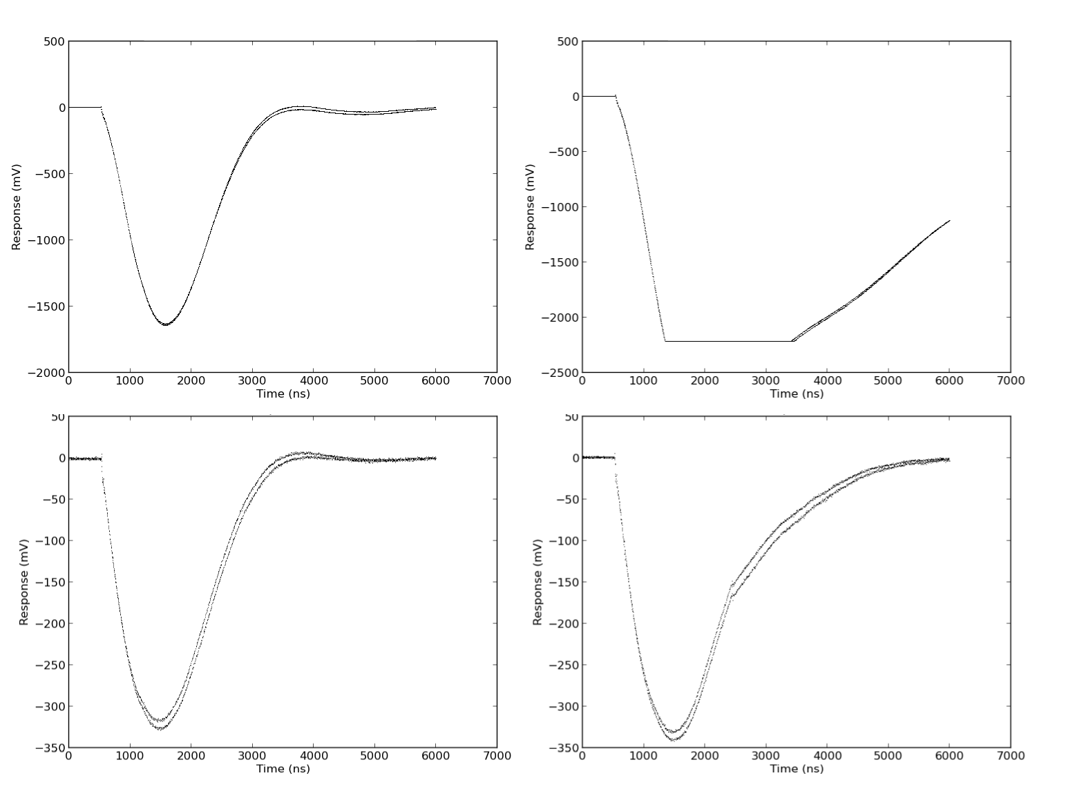
Figure 11: Four typical event curves corresponding to cosmics. Clockwise, starting top left: a regular curve, a clipped curve, a shallow curve where the two ADCs become distinguishable and a strange kink. Explanations may be found in the text.

Comparison of data rates with different Event Window sizes.¶
Overhead	Event Window	Event Window	Event Window	Frequency	Data rate
(bytes)	(samples)	(ns)	(bytes)	(Hz)	(kB/s)
25	3 / 6	15	18	31644	1361
25	11 / 22	55	66	11628	1058
25	21 / 42	105	126	6499	981
25	51 / 102	255	306	2793	925
25	101 / 202	505	606	1433	904
25	201 / 402	1005	1206	726	894
25	501 / 1002	2505	3006	293	888
25	801 / 1602	4005	4806	183	884
25	1201 / 2402	6005	7206	122	882
25	1601 / 3202	8005	9606	92	886
25	2000 / 4000	10000	12000	73	878

5.4.5. Summary¶

The results on the new CaloDAQ system can be summed up as follow:

The event acquisition rate exceeds the desired 120Hz by a wide margin. Using analog signal preprocessing so that only a few samples are necessary for an accurate representation of the energy captured by the calorimeter, rates up to 30kHz are a possibility.
The software performs very robustly at higher rates and extended data taking runs, although a serious test of the combination of the two still needs to be performed.
An offline message parser outputs various kinds of graphs, easily configurable.
The dynamic range and quality of the acquired data seems in order. The ADC alignment could be better tuned however, and the exact source for the kink must be discovered.
Changes in the HiSparc firmware may increase the acquisition rate even further. Switching off the second channel and lowering the sampling rate seem easily implemented.

5.5. Trigger¶

Now that the calorimeter data can be acquired at sufficiently high rates, it is time to optimize the trigger so that it can actually can deliver a reliable rate in the vicinity of 120Hz. Previously, when the busy signal of the RelaxD was not used, a timer set to ~500ms was used to both give the RelaxD time to fully complete the readout of an event and to compensate for trigger delays. Three important things were changed:

The trigger delays would be shortened as much as possible by using short cables.
The default state of the system would be acquisition mode on, instead of off.
The busy out of the RelaxD board would be incorporated in the trigger as the signal that dictates the start and end of a readout, and therefore no acquisitions.

The latter two are discussed below.

5.5.1. Changing the default state¶

Within the Detector R&D group, work was being done on a trigger incorporating a GridPix that was built with the only (theoretically) limiting factor: the GridPix readout process at 120Hz. As has been seen in the previous section, the calorimeter DAQ was designed with a continuously sampling ADC. The device keeps a 10μs buffer, which provides plenty of history to select the appropriate window for our uses. Moreover, it allows data taking without dead time. The GridPix has a certain dead-time (7-15 ms) when it receives the end of a shutter signal. After the end of a shutter, all pixel data is unloaded from the TimePix chip and transmitted to the computer by the RelaxD board. During this time, the chip can not acquire new event data, so a trigger should take this into account. Secondly, there is time lost in executing the trigger logic between the passing particle and the commencement of the GridPix readout. As stated in Tsopelas (2011), this translates to a small offset in track height. This is easy to correct for, but the data not recorded during the time it takes to execute the trigger logic is lost. The default state of the GridPix was therefore changed from off to on. By default, the GridPix is collecting data, and only when a trigger is received is data collection ceased and readout started. This trigger is then delayed to allow the electrons and ions to drift and induce a charge in the TimePix chip. The drift time is fortunately much larger than the time it takes to execute the trigger logic, so no data is lost and no offset should be introduced.

5.5.2. Utilizing the Busy signal¶

The second improvement is the incorporation of the RelaxD busy signal. This signal precisely determines the dead time during readout and will be used to block new hits during this period. Previously the busy signal was not used, but instead a relatively large delay with a timer. This delay was about half a second, which agrees nicely with the observed 2Hz acquisition rate in November. Occasionally the RelaxD board fails to correctly switch to acquisition mode, and will not recover by itself. Fortunately, when this happens, the busy signal is never activated and the RelaxD is reset by switching the shutter back on. A fallback timer, analogous to the delay timer as used in November, creates the automatic reset for that scenario, and could be set to a similar value as before: 500ms. The CaloDAQ trigger is for this reason connected to the busy out of the RelaxD: it never transmits an event to the computer if the RelaxD doesn’t, so that we don’t have to filter for incomplete events with only calorimeter data.

The new trigger design makes full use of the busy signal to decrease acquisition dead time as much as possible for a large majority of all incoming triggers. The dead time in a successful readout action is 7-15ms, so one can see how this is a major improvement over 500ms. For comparison: if we want to be able to maintain a 120Hz acquisition rate, one readout event must take no longer than 8.3ms.

5.5.3. Trigger logic¶

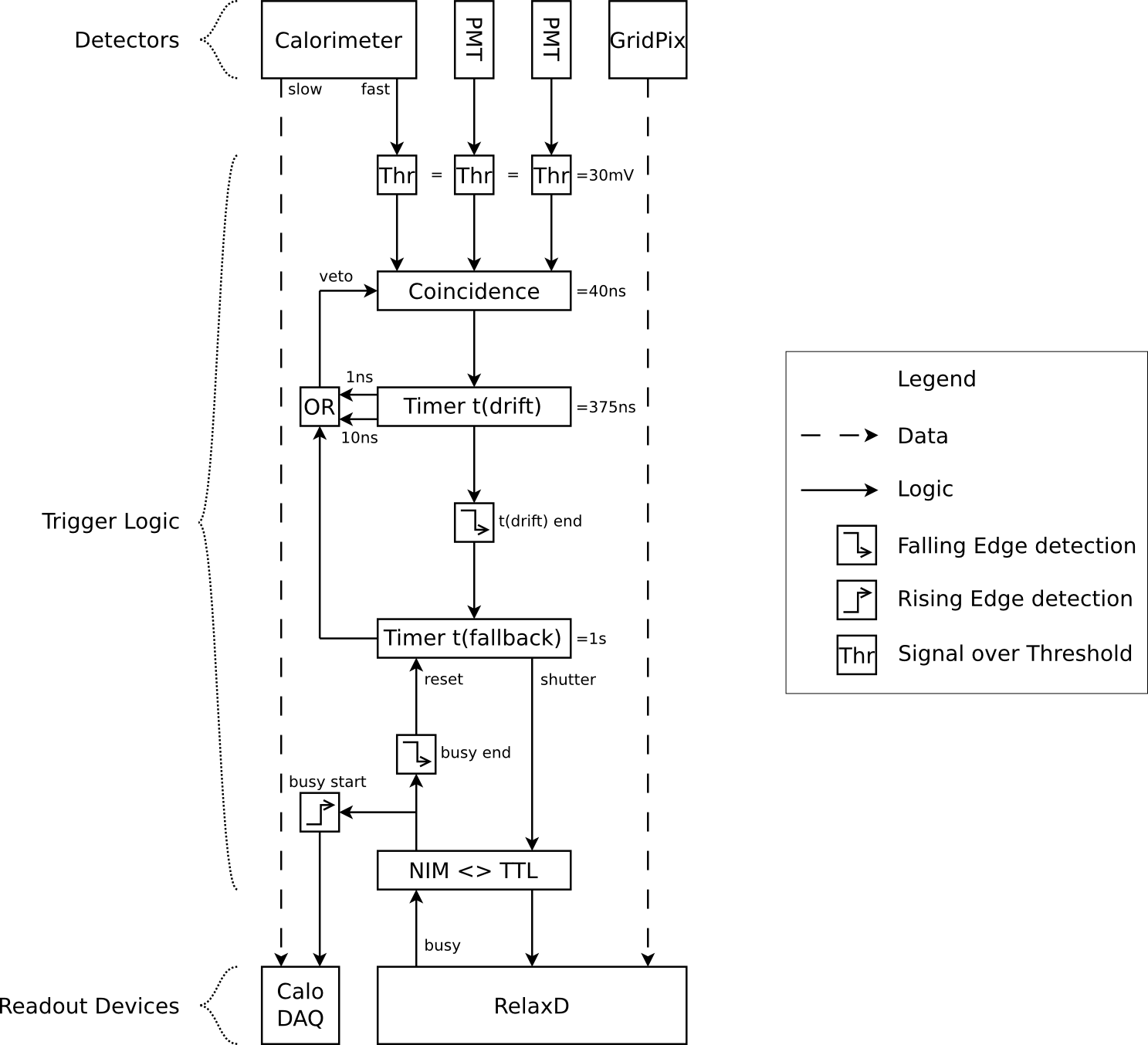
Figure 12: Overview of the trigger logic and its implementation. The Falling Edge detection between the timers is implemented by using the End-port of the drift timer. The other two Edge detections are implemented by a single coincidence.

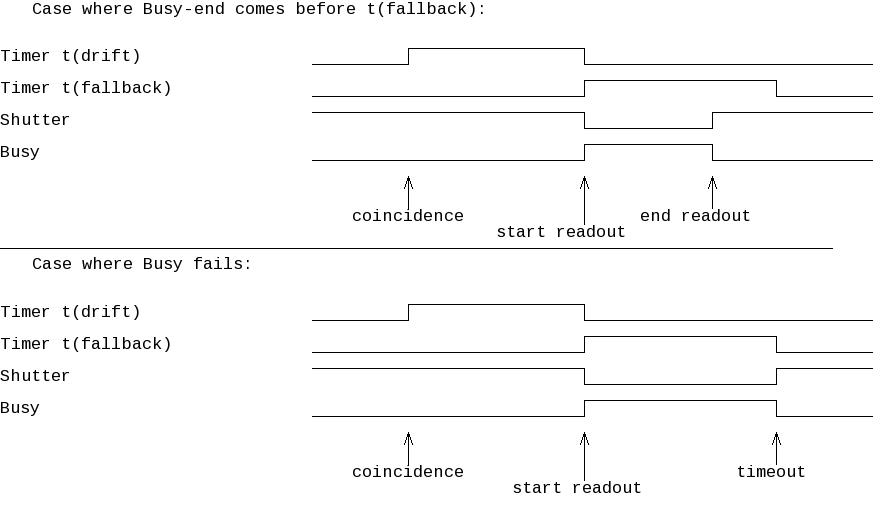
Figure 13: Trigger timing. The drift timer allows the ionized gas and electrons to drift, and is set to the top-to-bottom theoretical drift time based on Kopperts simulations. The readout stops when either the RelaxD board stops sending out a busy signal, or when the fallback timer has elapsed. The fallback timer was inserted to reset the system after occasional problems with the RelaxD that cause it to ‘hang’. The fallback timer prevents us from down time and an otherwise incomplete acquisition, by forcing the system out of this state if it lasts too long.

Commencing a data taking run starts with switching the system into acquisition mode. Currently, this is done by waiting for the first event, which can be generated artificially. The end of this event results in the shutter to be opened by default. The triple coincidence unit has a window of 40ns. If this condition is met, the drift timer ( $t_{drift}$ ) is started, to allow the electrons generated by the proton to drift towards to chip and induce charge in the TimePix chip. When the drift timer elapses, a second timer ( $t_{fallback}$ ) is started. Upon starting this second timer, it closes the shutter for the RelaxD board, which should cause it to start readout immediately. The busy output of the RelaxD will switch on: it should always be the opposite of the shutter. The start of the busy is used to trigger the CaloDAQ, and the end of the busy is used to reset the fallback timer. The fallback timer reopens the shutter when either its timer elapses or the end of the RelaxD busy resets it. It then releases the veto on the coincidence unit so that data acquisition is resumed. While two timers are running, the system is either waiting for the electrons to drift or for the data acquisition to finish. These two timers therefore veto the coincidence unit and thus the acceptance of new events.

For the final design we decided a triple coincidence between two small scintillators and the $BaF_2$ fast out would be the best way to exclude noise hits. Another detail is that the drift timer is connected to the OR-port twice: with a short (1ns) cable and with a longer 10ns cable. This is done to bridge the ~6-8ns it takes for the signal to arrive in the fallback timer and to start sending out its signal to the OR-port. Since the coincidence rates can be quite high, this small window was enough to accept new events which upset the proper acquisition of events.

In the figure 12 the trigger schematic is shown. The timing diagram is visible in figure 13.

5.5.4. Trigger verification¶

Initially the trigger was tested on a single frequency generator. This is only a partial test: first it will not generate jitter and second it does not test the triple coincidence. It was selected nonetheless, because a frequency generator that also could produce jitter was not available, and no two or three frequency generators were available or properly configurable for a reliable coincidence. The single frequency generator did however show that the trigger logic could be stably operated with rates up to 100kHz, which puts us far above the previous rate of 2Hz and far above the maximum acquisition rate of the GridPix. The triple coincidence was tested on a lower rate using cosmic rays: both scintillators and the calorimeter provided the proper coincidence. The acquisition rate in the calorimeter DAQ and the hit counter in the electronics rack kept proper synchronization during multiple multi-day test runs, and generated no noise hits. This test run was also a test of the calorimeter data acquisition quality: curves with the correct shape and magnitude that can be expected from cosmics were produced. The last test the trigger was subjected to was the single coincidence of the noise of the calorimeter. This produced event rates of about a 100Hz, and would test everything except the coincidence unit. Unfortunately an as of yet unresolved bug in the RelaxDAQ software did not allow for an extended test run at high rate: the software would crash on our machine after having recorded about 9000 events. By prematurely stopping the acceptance of new events, synchronicity could be tested for high rates during 2-3 minutes. During these very short high rate runs synchronicity between RelaxDAQ and CaloDAQ was kept; a promising result. Once the software bug in RelaxDAQ is resolved, an extended high rate run should be the last test before a new run at the proton accelerator at KVI.

5.5.5. Summary¶

The efforts on improving the trigger system have resulted in the following:

The full setup has been tested with cosmics for continuous multiday runs with 100% synchronicity and success.
The trigger with calorimeter data acquisition has been successfully tested up to an acquisition rate of 31kHz.
The full setup has been tested with 2-3 minute runs at an acquisition rate of ~70Hz with 100% synchronicity. 120Hz was not attained, and after discussion with the RelaxDAQ authors it was deemed a problem with the Linux build that should be fixable. The Windows build manages 120-130Hz for the RelaxDAQ authors.
The Linux build of RelaxDAQ must be fixed so that it does not crash after ~9000 events. The problem may partly lie with the RelaxD board as the firmware is in flux at the moment. Once fixed, an extended high speed run (an hour at 100Hz+) must be conducted to test whether or not the trigger keeps the two data channels in sync.
The design does not correct or block events with multiple particles. This means that bunch occupancy in the beam must remain as close to 1 as possible and the particle rate should still be kept within an order of magnitude or so of the desired acquisition rate (120Hz). The trigger provides only a logic block on new acquisitions, but not on new particles.

5.6. Conclusions¶

At the end of Chapter 4 some considerations were laid out for the eventual use of the setup in a medical context. Now we revisit these questions with our current abilities in mind.

How many protons do we need for an image?

Amaldi et al. (2011) write that $10^6$ usable proton tracks should be enough for a 100 by 100 $mm^2$ image. Scaled to the dimensions of our current GridPix drift volume, we would need 227k tracks.
What is the event acquisition rate that is required?

Amaldi et al. (2011) also write that the desired time for a full scan is in the order of a few seconds. If we take 10 seconds for example, this translates to an event acquisition rate of 27kHz. While the GridPix does not come close, a future version might. The TimePix version 3 is designed with a target pixel event acquisition rate of 40MHz which translates to an event acquisition rate of roughly 120kHz (a typical track had 100-300 pixel hits in our test run in November). Our new HiSparc based calorimeter ADC can manage an event acquisition rate of 31kHz, if a way is found to put an event with sufficient energy resolution in 6 samples.
How large is the beam spot?

While not investigated with the November data, for imaging a large spot is advantageous as speed is a more important consideration than spatial precision. Using a tracking plane before and after the patient, all the spatial information that is required should be provided.
What is the required beam current?

This depends greatly on the ability to handle multiple particles in one event. Since our calorimeter can measure only one residual energy value, any multi-particle event must be discarded. Tsopelas (2011) shows that a dependence of the number of ionizations per unit track length on the particle energy is visible, so perhaps this information can be used to select the track corresponding to the residual energy in the calorimeter in some cases. For the time being there is no experience with such a selection mechanism yet, which means that the beam current must translate to a proton rate no higher than the maximum event acquisition rate that the system can handle. At the moment this could be as high as 120Hz if the Linux RelaxDAQ problems are solved.
How many tracks can be correlated (before and after patient)?

Unfortunately multiple GridPix chips were not available, so correlation between before and after the patient is not possible at this time.
Scattering in strip detectors versus GridPix: is GridPix advantageous?

It is widely accepted that gas trackers scatter incident particles much less than solid state trackers, but no quantitative comparison has been performed at this time in the context of medical imaging.